Appearance
Running a simulation
A simulation (or transient run) steps your circuit forward in time and records the signals you asked for. This page covers the toolbar controls, how to start and stop a run, what the progress and warnings mean, and where the results show up.
New to the app? Build something first with The canvas, or follow Your first circuit end to end.
The simulation controls
Everything you need to run is in the middle of the top bar.

| Control | What it does |
|---|---|
| Run (▶) | Starts a transient simulation. Turns into a Stop button (■) while a run is in flight. |
| Run load flow (⚡) | Solves the steady-state load flow instead of a transient run. Disabled while a simulation is running. |
| Time Step | The integration step. Defaults to 50 µs. Smaller steps resolve faster dynamics but take longer to run. |
| Duration | How much simulated time to run. Defaults to 0.2 s. |
Each time field has a unit selector — s, ms, µs, or ns — so you can type 50 next to µs rather than 0.00005. The fields are locked while a run is active; stop the run to change them.
Choosing the time step and duration
The time step decides what the run can see; the duration decides how long it watches. A few rules of thumb cover most circuits:
- Resolve the fastest thing you care about. Find the shortest period in the circuit — a switching period, a ringing frequency, a control loop's fastest time constant — and use at least 20 to 50 steps per period. A 10 kHz converter (100 µs period) wants 2–5 µs; a 60 Hz network with nothing faster is comfortable at 50 µs.
- Transmission lines set a hard limit. A travelling-wave line needs the time step to be no longer than the travel time of the shortest line, and works best when the travel time is close to a whole number of steps. The run warns you when it isn't — see Chapter 9 of the EMT course.
- Control time constants must be longer than the step. A filter or lag whose time constant is shorter than half a step is unstable. If you don't need that dynamic, set its time constant to zero instead of shrinking the step.
- Check by halving. Run once, halve the time step, and run again. If the waveform you care about doesn't change visibly, the first step was small enough.
- Duration: start to steady state, plus the event. Leave enough time for the circuit to settle before a fault or switching event, and enough after it to see the response die out. Ramping the sources (a source's t_ramp) or starting from a load flow shortens the settling part.
Run time grows with duration divided by time step, so a 10 s study at 1 µs is ten million steps. If only part of the circuit needs the fine step, put that part in a subsystem running at a finer rate.
Record something first
A run only records signals that have a name — the observables. Before you run, make sure at least one signal is named, for example:
- double-click a wire and give it a name, or
- turn on a measurement (such as Measure current) in a component's properties dialog.
Then place an Oscilloscope, a Plot or a Meter and pick that signal to see it (see Displays). If nothing is named, the run still executes, but there's nothing to draw (see the warning below).
Starting a run
Click Run. Before stepping, NumaSim validates the circuit:
If there are blocking errors (an unpaired transmission line, a duplicate signal name, and so on), the run is refused and a message appears:
Cannot start simulation: N circuit validation error(s). Fix them and press Run again.
Click Show logs to see each problem; many entries highlight the offending component on the canvas when clicked.
If validation passes, the engine initializes and starts stepping. A progress bar appears under the toolbar and walks through its phases:
- Initializing… — setting up the run (allocating state).
- Running… — stepping, before the first block of results drains.
- 21% — determinate progress once results are streaming. While running, a secondary line shows the speed as a multiple of real time (e.g.
1.84× realtime).

To end a run early, click Stop (■). The bar shows Stopping…, then Stopped at the percentage it reached; whatever was computed so far stays on the displays. If a run fails, the bar shows Error and the details land in the logs.
"Nothing is being recorded"
If you run with no observables, the simulation still runs but warns you that it won't produce any plots:
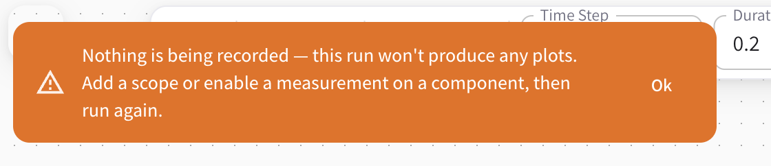
Nothing is being recorded — this run won't produce any plots. Add a scope or enable a measurement on a component, then run again.
Name a wire or turn on a measurement, then run again to get traces.
Reading the results
Results appear the moment they start streaming — you don't wait for the run to finish. They show up in the display components on your canvas:
- Oscilloscope — double-click it to open a floating panel of sub-plots you can zoom and pan while data streams.
- Plot — a chart drawn right on the canvas.
- Meter — the latest value of one signal, as a number.
See Displays for how to set each one up.
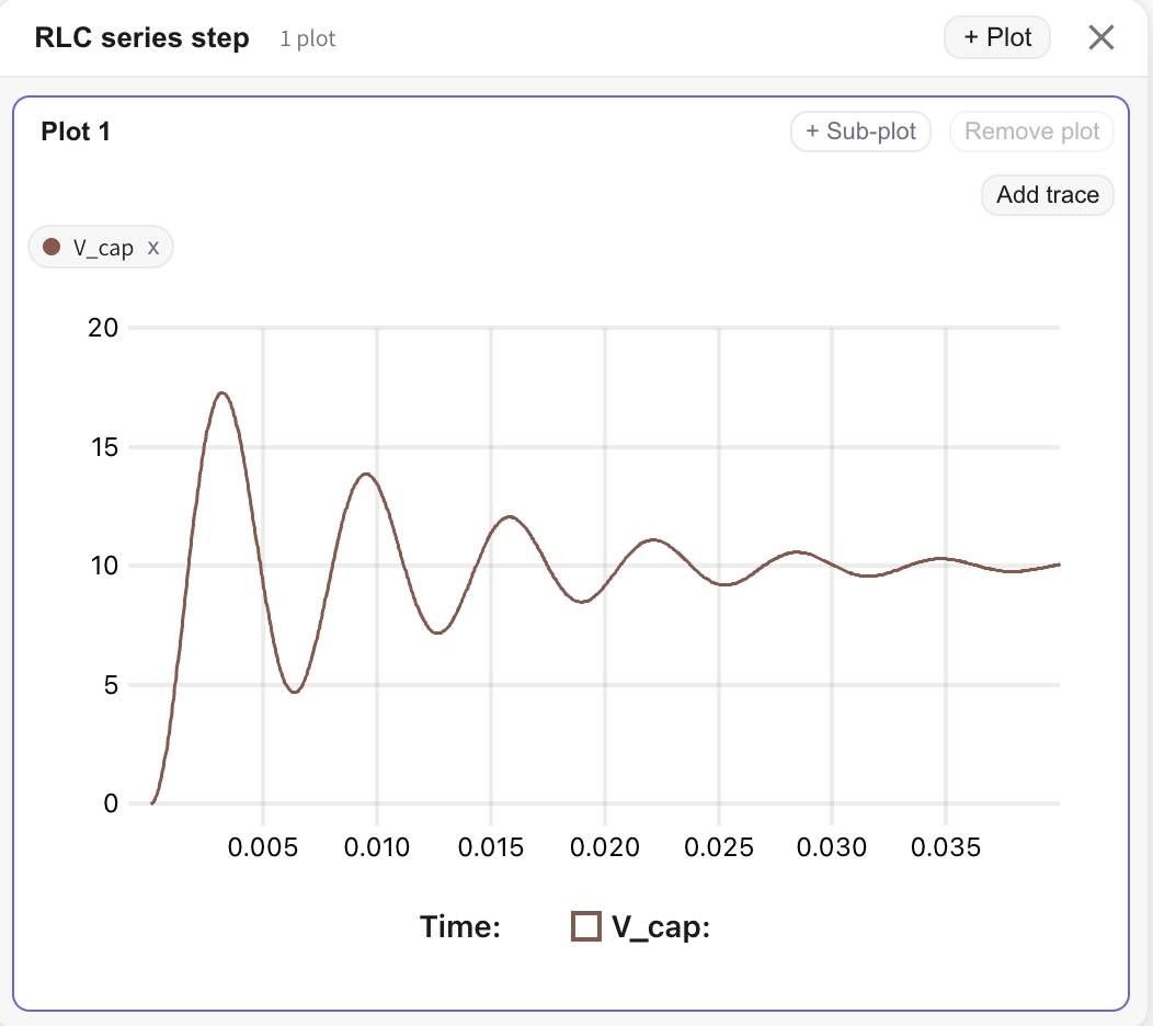
Each click of Run shows one run at a time and replaces the previous data — the traces you picked are kept, only the samples behind them are refreshed. NumaSim doesn't export results to a file, so to compare two runs, change one thing at a time and watch the displays.
When every run repeats a long settling period before the part you're studying, save a snapshot once and start later runs from it.
Where the run happens
The simulator runs locally in your browser — nothing leaves your machine.
Logs
Click Logs in the status bar at the bottom (next to Parameters) to open the Logs panel. It collects engine messages, validation errors, and warnings for the current run — the first place to look when a run is refused or a result looks wrong.
- Pick a log level in the menu next to the title (from Trace, the most detailed, to Error) to hide the less important messages.
- Click an entry that names a component to highlight it on the canvas.
- Use Copy filtered logs to paste the messages into a bug report, or Clear logs to start fresh. The panel also clears itself at the start of each run.
See also
- The canvas — build and place components.
- Snapshots — save a run's state and start later runs from it.
- Observables — declare what gets recorded.
- Displays — the Oscilloscope, Plot and Meter.
- Load flow — solve the steady state with the ⚡ button instead of a transient run.